
Exploring the unknown requires tolerating uncertainty.
Brian Greene
The science of Uncertainty Quantification (UQ) describes the propagation of uncertainty in dynamical systems and its major goal is to determine the likelihood of certain outcomes of dynamical systems, given some aspects of dynamical systems to not be exactly known. In other words, UQ provides mathematical tools to characterize the behavior of outputs of dynamical systems, given some sources of uncertainties involved in their structure.
In general, there exist two different categories of uncertainty: Aleatoric uncertainty and Epistemic uncertainty. Aleatoric uncertainty represents the randomness in physical phenomena, while epistemic uncertainty accounts for ignorance in accurate modeling of physical phenomena. The major difference between aleatory and epistemic uncertainty is that the aleatory uncertainty can not be reduced and it can only be better characterized, while epistemic uncertainty can be diminished by collection of information about the system under study.
The very first step to characterize the uncertainty of dynamical systems is to quantify the model output uncertainty in presence of epistemic uncertainty, e.g. presence of uncertain parameters or initial condition in model structure. This is also denoted as uncertainty propagation or uncertainty quantification.
There exist numerous techniques to perform the task of uncertainty quantification of dynamic systems in presence of uncertain parameters and/or initial conditions, ranging from simple Monte Carlo (MC) method to spectral decomposition based methods, like stochastic finite element and generalized Polynomial Chaos (gPC), and solution of Fokker-Planck-Kolmogorov Equation (FPKE). One should note that the choice of each method for uncertainty quantification depends on desired level of accuracy and available computational resources.
Ideally, Kolmogorov equation provides exact solution for propagation of uncertainty through dynamical systems that are in presence of parametric and/or model input uncertainties. Exact analytical description of uncertainty, provided by Kolmogorov equation, makes this approach very elegant candidate for uncertainty quantification of dynamical system. However, solving Kolmogorov equation is not usually straightforward. Unfortunately, exact solution of Kolmogorov equation is not attainable other than very few cases. Hence, alternative methods are proposed to approximate the solution of Kolmogorov equation.
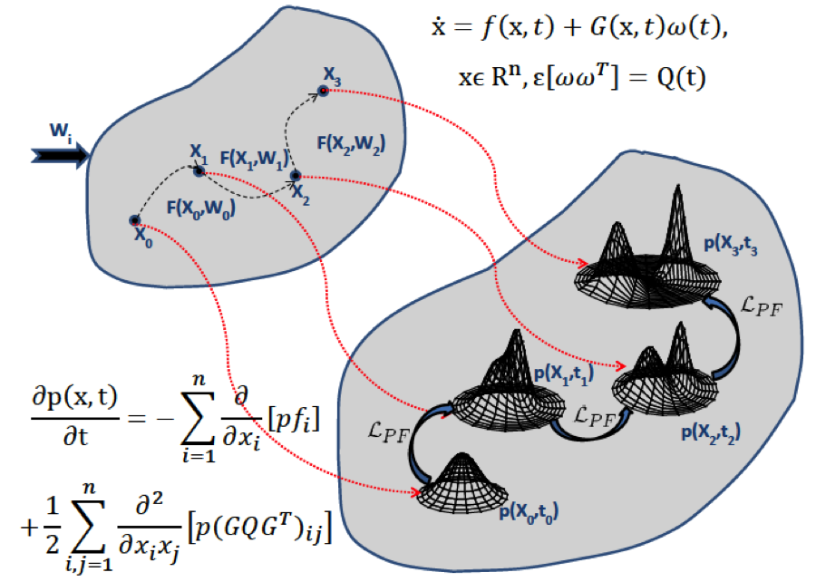
Fokker-Planck-Kolmogorov Equation provides accurate solution for spatiotemporal variations of probability density function
Unfortunately there exists significant computational cost involved in proposed approximate methods which restricts their applicability. Also, in higher dimensions, the computational cost involved in these methods becomes prohibitive. Hence, these methods can not be used to large scale systems.
On the other hand, Monte Carlo method is one of the most simplistic approaches that is widely used for uncertainty quantification of dynamical systems. In Monte Carlo method, a large set of points are generated based on distribution of uncertain parameter/initial conditions. Generated random points are then propagated through dynamic model to approximate statistics of model output in future time steps. However, ease of implementation and simplicity of MC approach makes it a very desirable candidate for uncertainty quantification of dynamical system, but its low rate of convergence hinders its applicability when a precise approximation of model output uncertainty is needed. In other words, depending on involved nonlinearities, a large number of random points need to be propagated through dynamic model to ensure convergence of obtained statistics. Clearly, larger number of MC samples results in more accurate statistics, but it results in more computational load at the same time which is undesirable. Schematic view of Monte Carlo method is shown in the following figure.
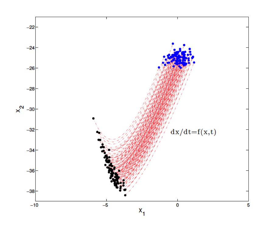
Schematic illustration of Monte Carlo approach
Spectral decomposition based techniques are another set of tools that are often used to avoid computational burden of Monte Carlo approach in uncertainty quantification of dynamic systems. The essence of spectral decomposition methods lies in decomposition of uncertain variable into a linear combination of a set of basis functions which are function of standardized random variable = [ζ1, ζ2, … ,ζm ], where m is the number of existing independent uncertain variables in dynamic model. The major benefit of spectral decomposition based methods is their low computational cost and their ease of implementation. However, convergence issues in presence of severe nonlinearities, large number of independent uncertain variables, and long time uncertainty propagation restrict applicability of spectral decomposition methods.
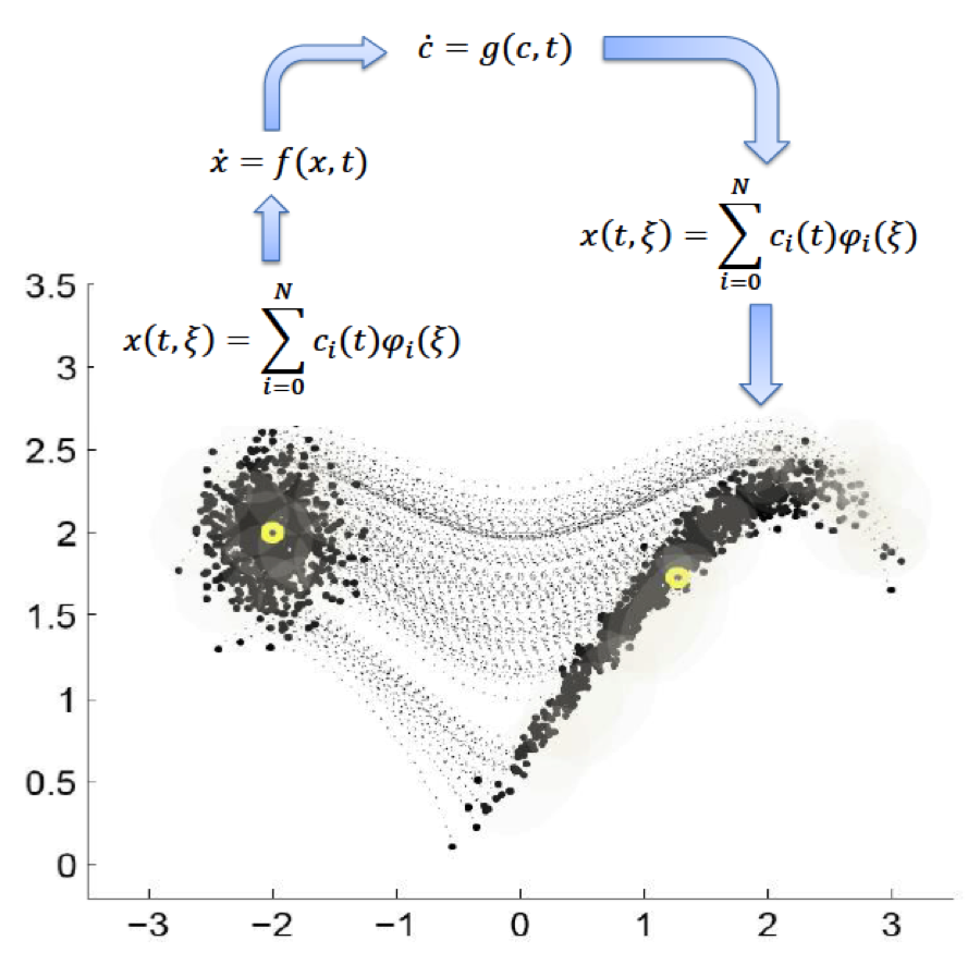
Spectral decomposition approach vs. Monte Carlo method
An alternative approach to perform the task of uncertainty quantification is to make use of quadrature points. In quadrature points method, a set of intelligently selected points will be propagated through dynamical model (which can be given as a black-box model or a set of dynamical equations) and statistics of the output (e.g. mean and variance) are then determined by weighted average of model outputs. The major benefit of quadrature scheme is its significantly less computational cost with respect to Monte Carlo method. Also, the computational complexity involved in quadrature methods is far less than the computational complexities involved in solution of Kolmogorov equation. In addition, quadrature method can be combined with spectral decomposition based methods like gPC theory to improve their performance.
To summarize our discussion, a comparison between discussed methods is provided in the following figure. As one can see, method of quadrature points requires the minimal computational effort, while at the same time it provides reasonable degree of accuracy, comparing with other methods.
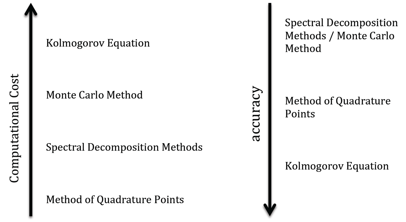
Comparison between different applied methods for uncertainty quantification
